Variational Basis State Encoder (Ground State)
1 Backgroud
This tutorial is for variational basis state encoder (VBE) for the ground state of the Holstein model.
To calculate the ground state of Holstein model accurately, many levels of phonons are needed, which will cost too many qubits in quantum circuit. There exists another idea that we can view linear conbination of phonons as an effective phonon mode, which is possible to save the qubits in phonon encoding:
Here, we transform the original phonon basis \(\ket{m}\) to the encoded basis \(\ket{n}\), via transformation operator \(\hat{B}[l]\). The form of \(\hat{B}[l]\) is the central of VBE and the algorithm are presented in section 2. For more details, see https://doi.org/10.1103/PhysRevResearch.5.023046
2 Algorithm Realization
2.1 Imports
[1]:
import numpy as np
import scipy
from opt_einsum import contract
import tensorcircuit as tc

from tencirchem import set_backend, Op, BasisSHO, BasisSimpleElectron, Mpo, Model
from tencirchem.dynamic import get_ansatz, qubit_encode_op_grouped, qubit_encode_basis
from tencirchem.utils import scipy_opt_wrap
from tencirchem.applications.vbe_lib import get_psi_indices, get_contracted_mpo, get_contract_args
2.2 Initial setups
In this section, we set intital parameters for coming sections. Here, JAX is used as backend. nsite, omega, v correspond to the site number, phonon frequency \(\omega\), transfer intergral \(V\) in Holstein model, respectively:
Each site possesses one phonon mode, which is represented by 2 qubit per phonon (see n_qubit_per_mode). Considering gray encoding is adopted, the number of phonon basis (nbas_v) is \(2^2\). psi_index_top and psi_index_bottom correspond to the physical index of ket and bra, b_dof_vidx correspond to the qubits that need VBE, psi_shape2 is the physical bond dimension of each qubit state. The stucture of wavefunction and operator are presented in Fig.1. Note that the
related arguments and functions are also marked.  Fig. 1 The structure of wavefunction and operator. Blue squares correspond to qubit representing spin, green circles correspond to qubits representing vibrations, purple circles correspond to \(B[l]\), and orange squares correspond to Matrix Product Operators (MPO).
[2]:
backend = set_backend("jax")

nsite = 3
omega = 1
v = 1
# two qubit for each mode
n_qubit_per_mode = 2
nbas_v = 1 << n_qubit_per_mode

# -1 for electron dof, natural numbers for phonon dof
dof_nature = np.array([-1, 0, 0, -1, 1, 1, -1, 2, 2])
# physical index for phonon mode
b_dof_pidx = np.array([1, 3, 5])

psi_idx_top, psi_idx_bottom, b_dof_vidx = get_psi_indices(dof_nature, b_dof_pidx, n_qubit_per_mode)

n_dof = len(dof_nature)
psi_shape2 = [2] * n_dof

print(
    "psi_index_top: ",
    psi_idx_bottom,
    "\n psi_index_bottom: ",
    psi_idx_bottom,
    "\n b_dof_vidx: ",
    b_dof_vidx,
    "\n psi_shape2: ",
    psi_shape2,
)

c = tc.Circuit(nsite * 3)  # generate quantum circuit
c.X(0)  # prepare one-electron initial state
n_layers = 3  # layers of ansatz
An NVIDIA GPU may be present on this machine, but a CUDA-enabled jaxlib is not installed. Falling back to cpu.
psi_index_top:  ['p-0-bottom', 'v-1-0-bottom', 'v-1-1-bottom', 'p-2-bottom', 'v-3-0-bottom', 'v-3-1-bottom', 'p-4-bottom', 'v-5-0-bottom', 'v-5-1-bottom']
 psi_index_bottom:  ['p-0-bottom', 'v-1-0-bottom', 'v-1-1-bottom', 'p-2-bottom', 'v-3-0-bottom', 'v-3-1-bottom', 'p-4-bottom', 'v-5-0-bottom', 'v-5-1-bottom']
 b_dof_vidx:  [array([1, 2]), array([4, 5]), array([7, 8])]
 psi_shape2:  [2, 2, 2, 2, 2, 2, 2, 2, 2]
2.3 Get Variational Hamiltonian Ansatz (VHA) Terms
In this section, we will generate variational hamiltonian ansatz terms. The following ansatz is adopted:
The anasatz is transformed from electron-phonon basis to qubit basis through qubit_encode_op_grouped() and qubit_encode_basis()
[3]:
def get_vha_terms():
    # variational Hamiltonian ansatz (vha) terms

    g = 1  # dummy value, doesn't matter
    ansatz_terms = []
    for i in range(nsite):
        j = (i + 1) % nsite
        ansatz_terms.append(Op(r"a^\dagger a", [i, j], v) - Op(r"a^\dagger a", [j, i], v))
        ansatz_terms.append(Op(r"a^\dagger a b^\dagger-b", [i, i, (i, 0)], g * omega))

    basis = []
    for i in range(nsite):
        basis.append(BasisSimpleElectron(i))
        basis.append(BasisSHO((i, 0), omega, nbas_v))

    ansatz_terms, _ = qubit_encode_op_grouped(ansatz_terms, basis, boson_encoding="gray")

    # More flexible ansatz by decoupling the parameters in the e-ph coupling term
    ansatz_terms_extended = []
    for i in range(nsite):
        ansatz_terms_extended.extend([ansatz_terms[2 * i]] + ansatz_terms[2 * i + 1])
    spin_basis = qubit_encode_basis(basis, boson_encoding="gray")
    return ansatz_terms_extended, spin_basis


ansatz_terms, spin_basis = get_vha_terms()
ansatz = get_ansatz(ansatz_terms, spin_basis, n_layers, c)

print(
    "ansatz_terms: \n",
    ansatz_terms,
    "\nspin_basis: \n",
    spin_basis,
    "\nansatz: \n",
    ansatz,
)
ansatz_terms:
 [[Op('X Y', [0, 1], 0.5j), Op('Y X', [0, 1], -0.5j)], Op('Y', [((0, 0), 'TCCQUBIT-1')], 0.1830127018922193j), Op('Z Y', [((0, 0), 'TCCQUBIT-0'), ((0, 0), 'TCCQUBIT-1')], -0.6830127018922193j), Op('Y', [((0, 0), 'TCCQUBIT-0')], -0.3535533905932738j), Op('Y Z', [((0, 0), 'TCCQUBIT-0'), ((0, 0), 'TCCQUBIT-1')], 0.3535533905932738j), Op('Z Y', [0, ((0, 0), 'TCCQUBIT-1')], -0.1830127018922193j), Op('Z Z Y', [0, ((0, 0), 'TCCQUBIT-0'), ((0, 0), 'TCCQUBIT-1')], 0.6830127018922193j), Op('Z Y', [0, ((0, 0), 'TCCQUBIT-0')], 0.3535533905932738j), Op('Z Y Z', [0, ((0, 0), 'TCCQUBIT-0'), ((0, 0), 'TCCQUBIT-1')], -0.3535533905932738j), [Op('X Y', [1, 2], 0.5j), Op('Y X', [1, 2], -0.5j)], Op('Y', [((1, 0), 'TCCQUBIT-1')], 0.1830127018922193j), Op('Z Y', [((1, 0), 'TCCQUBIT-0'), ((1, 0), 'TCCQUBIT-1')], -0.6830127018922193j), Op('Y', [((1, 0), 'TCCQUBIT-0')], -0.3535533905932738j), Op('Y Z', [((1, 0), 'TCCQUBIT-0'), ((1, 0), 'TCCQUBIT-1')], 0.3535533905932738j), Op('Z Y', [1, ((1, 0), 'TCCQUBIT-1')], -0.1830127018922193j), Op('Z Z Y', [1, ((1, 0), 'TCCQUBIT-0'), ((1, 0), 'TCCQUBIT-1')], 0.6830127018922193j), Op('Z Y', [1, ((1, 0), 'TCCQUBIT-0')], 0.3535533905932738j), Op('Z Y Z', [1, ((1, 0), 'TCCQUBIT-0'), ((1, 0), 'TCCQUBIT-1')], -0.3535533905932738j), [Op('X Y', [0, 2], -0.5j), Op('Y X', [0, 2], 0.5j)], Op('Y', [((2, 0), 'TCCQUBIT-1')], 0.1830127018922193j), Op('Z Y', [((2, 0), 'TCCQUBIT-0'), ((2, 0), 'TCCQUBIT-1')], -0.6830127018922193j), Op('Y', [((2, 0), 'TCCQUBIT-0')], -0.3535533905932738j), Op('Y Z', [((2, 0), 'TCCQUBIT-0'), ((2, 0), 'TCCQUBIT-1')], 0.3535533905932738j), Op('Z Y', [2, ((2, 0), 'TCCQUBIT-1')], -0.1830127018922193j), Op('Z Z Y', [2, ((2, 0), 'TCCQUBIT-0'), ((2, 0), 'TCCQUBIT-1')], 0.6830127018922193j), Op('Z Y', [2, ((2, 0), 'TCCQUBIT-0')], 0.3535533905932738j), Op('Z Y Z', [2, ((2, 0), 'TCCQUBIT-0'), ((2, 0), 'TCCQUBIT-1')], -0.3535533905932738j)]
spin_basis:
 [BasisHalfSpin(dof: 0, nbas: 2), BasisHalfSpin(dof: ((0, 0), 'TCCQUBIT-0'), nbas: 2), BasisHalfSpin(dof: ((0, 0), 'TCCQUBIT-1'), nbas: 2), BasisHalfSpin(dof: 1, nbas: 2), BasisHalfSpin(dof: ((1, 0), 'TCCQUBIT-0'), nbas: 2), BasisHalfSpin(dof: ((1, 0), 'TCCQUBIT-1'), nbas: 2), BasisHalfSpin(dof: 2, nbas: 2), BasisHalfSpin(dof: ((2, 0), 'TCCQUBIT-0'), nbas: 2), BasisHalfSpin(dof: ((2, 0), 'TCCQUBIT-1'), nbas: 2)]
ansatz:
 <function get_ansatz.<locals>.ansatz at 0x7fe2ab768670>
2.4 Cost Functions for VQE Part
The VQE parameters \(\theta_k\) are optimized via following equation:
where
[4]:
def cost_fn(params, h):
    state = ansatz(params)
    return (state.conj() @ (h @ state)).squeeze().real


vg = backend.jit(backend.value_and_grad(cost_fn))
opt_fn = scipy_opt_wrap(vg)
2.5 Get Hamiltonian Terms and Basis
In this section, we generate the operator of the Holstein Hamiltonian presented in Section 2.2. The format of the operator are shown in Fig. 1. Note that the number of phonon levels are controlled by nbas.
[5]:
def get_ham_terms_and_basis(g, nbas):
    terms = []
    for i in range(nsite):
        terms.append(Op(r"b^\dagger b", (i, 0), omega))
        terms.append(Op(r"a^\dagger a b^\dagger+b", [i, i, (i, 0)], g * omega))
        j = (i + 1) % nsite
        terms.append(Op(r"a^\dagger a", [i, j], -v))
        terms.append(Op(r"a^\dagger a", [j, i], -v))

    basis = []
    for i in range(nsite):
        basis.append(BasisSimpleElectron(i))
        basis.append(BasisSHO((i, 0), omega, nbas))

    return terms, basis
2.6 Update \(B[l]\) in Iteration
In this section, the function that calculates \(B[l]\) are defined:
where
and
The graphic representarion of h_contracted is presented in Fig. 2. Obiviously, if \(\hat{H}\) are provided, we can obtain \(\hat{B}[l]\) by solving the equation mentioned above. Considering this is a non-linear equation, several initial guesses are needed to avoid local minimum, which is controlled by nroot.  Fig. 2 Graphic representation of
 h_contracted
[6]:
def solve_b_array(psi, h_mpo, b_array, i):
    nbas = b_array.shape[-1]
    # get the input of tensor contraction function `contract`
    args = get_contract_args(psi, h_mpo, b_array, i, n_qubit_per_mode, psi_idx_top, psi_idx_bottom, b_dof_pidx)
    k = b_dof_pidx[i]
    # output indices
    args.append(
        [
            f"v-{k}-0-bottom",
            f"v-{k}-1-bottom",
            f"p-{k}-bottom",
            f"v-{k}-0-top",
            f"v-{k}-1-top",
            f"p-{k}-top",
            "mpo-0",
            f"mpo-{len(h_mpo)}",
        ]
    )
    # get contracted_h and reshape the dofs named v-{k}-0-bottom(top) and v-{k}-1-bottom(top) to one dof with dimension 4
    contracted_h = contract(*args).reshape(4, nbas, 4, nbas)
    nroot = 3

    def f(x):
        x = x.reshape(nroot, 4, nbas)
        # calculate P[l]
        p = contract("abc, abd -> acd", x.conj(), x)
        return contract("abcd, kab, kde -> kce", contracted_h, x, (np.array([np.eye(nbas)] * nroot) - p)).ravel()

    # solve the equation mentioned above to obtain B[l]
    sols = scipy.optimize.root(f, [b_array[i].flatten()] * nroot, method="df-sane").x.reshape(3, 4, nbas)

    sols = list(sols) + [b_array[i].copy()]
    b_array = b_array.copy()
    es = []
    for k, new_b in enumerate(sols):
        # ensure the orthomormal constraint of B[l]
        if not np.allclose(new_b @ new_b.T, np.eye(4)):
            # print(f"Enforcing orthogonality for the {k}th root of b_array[{i}]")
            new_b = np.linalg.qr(new_b.T)[0].T
        b_array[i] = new_b
        e = psi @ get_contracted_mpo(h_mpo, b_array, n_qubit_per_mode, b_dof_pidx, psi_idx_top + psi_idx_bottom) @ psi
        es.append(e)
    # print(np.array(es))
    lowest_id = np.argmin(es)
    return sols[lowest_id]
2.7 Main Structure of the Function
This section is the main part of the funtion. The codes contain following parts:
Initialize the parameters and functions, some initializations are also preformed in section 2.2
Search for ground state, where \(\theta_k\) are updated via VQE and \(B[l]\) are calculated via functions in Section 2.6.
[8]:
vqe_e = []
thetas = np.zeros(len(ansatz_terms) * n_layers)

for g in [1.5, 3]:
    for nbas in [4, 8, 12, 16, 20, 24, 28, 32]:
        print(f"g: {g}, nbas: {nbas}")

        # take gray encoding as an initial guess for `b_array`
        b_list = []
        for i in range(max(dof_nature) + 1):
            b = np.eye(nbas)[:nbas_v]  # nbas_dummy * nbas
            b_list.append(b)
        b_array = np.array(b_list)

        # initialize, get hamitonians and basis, see section 2.5
        terms, basis = get_ham_terms_and_basis(g, nbas)
        model = Model(basis, terms)
        h_mpo = Mpo(model)

        # searching for the ground state.
        for i_iter in range(10):
            h_contracted = get_contracted_mpo(
                h_mpo, b_array, n_qubit_per_mode, b_dof_pidx, psi_idx_top + psi_idx_bottom
            )
            # get \theta_k via VQE
            opt_res = scipy.optimize.minimize(opt_fn, args=(h_contracted,), x0=thetas / 2, jac=True, method="L-BFGS-B")
            print(f"Iter {i_iter} VQE energy: {opt_res.fun}")
            thetas = opt_res.x
            psi = np.array(ansatz(thetas).real)
            # Update b[l] via functions in section 2.6
            for i in range(len(b_array)):
                b_array[i] = solve_b_array(psi, h_mpo, b_array, i)
        vqe_e.append(opt_res.fun)

    print(vqe_e)
g: 1.5, nbas: 4
Iter 0 VQE energy: -3.1508416128890313
Iter 1 VQE energy: -3.1507858838816376
Iter 2 VQE energy: -3.1508608481716656
Iter 3 VQE energy: -3.150867173130474
Iter 4 VQE energy: -3.1507760219657097
Iter 5 VQE energy: -3.1508712542841204
Iter 6 VQE energy: -3.1508619663363584
Iter 7 VQE energy: -3.150862097675895
Iter 8 VQE energy: -3.1508558599533214
Iter 9 VQE energy: -3.1508452460745824
g: 1.5, nbas: 8
Iter 0 VQE energy: -3.150839580645302
Iter 1 VQE energy: -3.2066949093848724
Iter 2 VQE energy: -3.212971955811858
Iter 3 VQE energy: -3.21359027706454
Iter 4 VQE energy: -3.213786701570586
Iter 5 VQE energy: -3.213875852088408
Iter 6 VQE energy: -3.2139390416159745
Iter 7 VQE energy: -3.213949104011919
Iter 8 VQE energy: -3.213987256845763
Iter 9 VQE energy: -3.2152956996689386
g: 1.5, nbas: 12
Iter 0 VQE energy: -3.1506086065941177
Iter 1 VQE energy: -3.207291050935305
Iter 2 VQE energy: -3.2135257229321295
Iter 3 VQE energy: -3.2141699728510145
Iter 4 VQE energy: -3.2143365747584576
Iter 5 VQE energy: -3.214441211557893
Iter 6 VQE energy: -3.2149215057907408
Iter 7 VQE energy: -3.215021952188251
Iter 8 VQE energy: -3.2150830781181865
Iter 9 VQE energy: -3.2151588242226294
g: 1.5, nbas: 16
Iter 0 VQE energy: -3.151275240878887
Iter 1 VQE energy: -3.2070935536922067
Iter 2 VQE energy: -3.2136287739682468
Iter 3 VQE energy: -3.2143020839991756
Iter 4 VQE energy: -3.2144651007997775
Iter 5 VQE energy: -3.2145842050117097
Iter 6 VQE energy: -3.2146841025772996
Iter 7 VQE energy: -3.21479318479846
Iter 8 VQE energy: -3.2148943236005287
Iter 9 VQE energy: -3.2149540916947945
g: 1.5, nbas: 20
Iter 0 VQE energy: -3.151289122850235
Iter 1 VQE energy: -3.207014859265433
Iter 2 VQE energy: -3.2132344731718514
Iter 3 VQE energy: -3.2141907479392553
Iter 4 VQE energy: -3.2143546694580207
Iter 5 VQE energy: -3.214450278123804
Iter 6 VQE energy: -3.2145674514358706
Iter 7 VQE energy: -3.2146390373914153
Iter 8 VQE energy: -3.2150470541341685
Iter 9 VQE energy: -3.215173127034174
g: 1.5, nbas: 24
Iter 0 VQE energy: -3.150827151041051
Iter 1 VQE energy: -3.207129572687281
Iter 2 VQE energy: -3.2137825485777864
Iter 3 VQE energy: -3.2144545350583797
Iter 4 VQE energy: -3.214629617805067
Iter 5 VQE energy: -3.214737029069743
Iter 6 VQE energy: -3.214830643223987
Iter 7 VQE energy: -3.2149177270776037
Iter 8 VQE energy: -3.215007843231478
Iter 9 VQE energy: -3.2150878222798105
g: 1.5, nbas: 28
Iter 0 VQE energy: -3.1513226796412654
Iter 1 VQE energy: -3.206975159802363
Iter 2 VQE energy: -3.21360025168811
Iter 3 VQE energy: -3.2143725838746917
Iter 4 VQE energy: -3.2145131528688684
Iter 5 VQE energy: -3.214604325896769
Iter 6 VQE energy: -3.2146927550103013
Iter 7 VQE energy: -3.214787435576051
Iter 8 VQE energy: -3.2148807292126254
Iter 9 VQE energy: -3.214950439086758
g: 1.5, nbas: 32
Iter 0 VQE energy: -3.1508096031820507
Iter 1 VQE energy: -3.206930098390965
Iter 2 VQE energy: -3.213589086530922
Iter 3 VQE energy: -3.214254153558814
Iter 4 VQE energy: -3.2143964407024552
Iter 5 VQE energy: -3.2144846301084025
Iter 6 VQE energy: -3.2145623430858894
Iter 7 VQE energy: -3.214620531205786
Iter 8 VQE energy: -3.2147225823351513
Iter 9 VQE energy: -3.2147844815701507
[-3.1508452460745824, -3.2152956996689386, -3.2151588242226294, -3.2149540916947945, -3.215173127034174, -3.2150878222798105, -3.214950439086758, -3.2147844815701507]
g: 3, nbas: 4
Iter 0 VQE energy: -5.970095373880274
Iter 1 VQE energy: -5.97011140752757
Iter 2 VQE energy: -5.970112221832909
Iter 3 VQE energy: -5.970097206562884
Iter 4 VQE energy: -5.970097522226955
Iter 5 VQE energy: -5.970084918795675
Iter 6 VQE energy: -5.97009612094958
Iter 7 VQE energy: -5.970090087724759
Iter 8 VQE energy: -5.970084917787736
Iter 9 VQE energy: -5.970092472244904
g: 3, nbas: 8
Iter 0 VQE energy: -5.970078968351394
Iter 1 VQE energy: -7.563619315159238
Iter 2 VQE energy: -7.86542656566074
Iter 3 VQE energy: -7.88623299324116
Iter 4 VQE energy: -7.8756160081347755
Iter 5 VQE energy: -7.87669855576027
Iter 6 VQE energy: -7.8770414783544185
Iter 7 VQE energy: -7.877214342205345
Iter 8 VQE energy: -7.877399262407691
Iter 9 VQE energy: -7.877447749293062
g: 3, nbas: 12
Iter 0 VQE energy: -5.970404607808003
Iter 1 VQE energy: -8.210512264715195
Iter 2 VQE energy: -8.734258414528332
Iter 3 VQE energy: -8.761817418245505
Iter 4 VQE energy: -8.764385439689185
Iter 5 VQE energy: -8.765150683117824
Iter 6 VQE energy: -8.765371623528338
Iter 7 VQE energy: -8.765594133409062
Iter 8 VQE energy: -8.765731045348685
Iter 9 VQE energy: -8.765868762122404
g: 3, nbas: 16
Iter 0 VQE energy: -5.968823174685871
Iter 1 VQE energy: -8.433088894554963
Iter 2 VQE energy: -9.027450708952731
Iter 3 VQE energy: -9.056048877152831
Iter 4 VQE energy: -9.057310249886191
Iter 5 VQE energy: -9.057405427978866
Iter 6 VQE energy: -9.057711262240172
Iter 7 VQE energy: -9.057977529966319
Iter 8 VQE energy: -9.058229991701616
Iter 9 VQE energy: -9.058429201135686
g: 3, nbas: 20
Iter 0 VQE energy: -5.948528657871584
Iter 1 VQE energy: -8.368829839591752
Iter 2 VQE energy: -9.083438191408403
Iter 3 VQE energy: -9.11436452030949
Iter 4 VQE energy: -9.115669532398497
Iter 5 VQE energy: -9.115868599561257
Iter 6 VQE energy: -9.116043601598792
Iter 7 VQE energy: -9.116167929411532
Iter 8 VQE energy: -9.11643438333657
Iter 9 VQE energy: -9.116603277604245
g: 3, nbas: 24
Iter 0 VQE energy: -5.947042292691847
Iter 1 VQE energy: -8.365954455675366
Iter 2 VQE energy: -9.03656892084732
Iter 3 VQE energy: -9.11649389980292
Iter 4 VQE energy: -9.12039969438638
Iter 5 VQE energy: -9.120853070374695
Iter 6 VQE energy: -9.121044950929027
Iter 7 VQE energy: -9.121198735794241
Iter 8 VQE energy: -9.121394623009978
Iter 9 VQE energy: -9.12156465701712
g: 3, nbas: 28
Iter 0 VQE energy: -5.94852290058614
Iter 1 VQE energy: -8.373669662264637
Iter 2 VQE energy: -9.077430296028782
Iter 3 VQE energy: -9.118353243461202
Iter 4 VQE energy: -9.120646592845254
Iter 5 VQE energy: -9.121017986552905
Iter 6 VQE energy: -9.121200880818158
Iter 7 VQE energy: -9.121406754497627
Iter 8 VQE energy: -9.12160334523664
Iter 9 VQE energy: -9.121785885087258
g: 3, nbas: 32
Iter 0 VQE energy: -5.955856129341857
Iter 1 VQE energy: -8.411614122038424
Iter 2 VQE energy: -9.013222667482161
Iter 3 VQE energy: -9.115359115707335
Iter 4 VQE energy: -9.120333885780456
Iter 5 VQE energy: -9.12077712341391
Iter 6 VQE energy: -9.120890286646729
Iter 7 VQE energy: -9.120977919424327
Iter 8 VQE energy: -9.121046355348854
Iter 9 VQE energy: -9.121145181818363
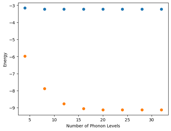
[-3.1508452460745824, -3.2152956996689386, -3.2151588242226294, -3.2149540916947945, -3.215173127034174, -3.2150878222798105, -3.214950439086758, -3.2147844815701507, -5.970092472244904, -7.877447749293062, -8.765868762122404, -9.058429201135686, -9.116603277604245, -9.12156465701712, -9.121785885087258, -9.121145181818363]
[9]:
# plot the results
from matplotlib import pyplot as plt

nbas = [4, 8, 12, 16, 20, 24, 28, 32]
plt.scatter(nbas, vqe_e[0:8], label="g=1.5")
plt.scatter(nbas, vqe_e[8:], label="g=3.0")
plt.xlabel("Number of Phonon Levels")
plt.ylabel("Energy")
[9]:
Text(0, 0.5, 'Energy')